Formula Hybrid Battery Cooling System Design and Optimization Project
Contributors: Matthew Galarza
Introduction
The growing trend towards environmentally-friendly and energy-efficient society has shifted the focus of automotive manufacturers from internal combustion (IC) engines to battery-powered electric motors. Although offering superior efficiency and reduced greenhouse gas (GHG) emissions, electric vehicles have a few areas that require improvement in order to overtake IC engines in the field of ground transportation. These areas are fuel energy density, material rarity and recyclability, and cost. An additional area of concern is battery cooling, as batteries are more temperature sensitive than their non-electric counterparts.
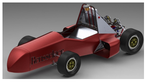
The goal of this project is to address the last area discussed above, battery cooling systems. The battery cooling system designed will be for a Formula Hybrid vehicle with the objectives of fitting within specified dimensions and reduced complexity. A figure of a proposed vehicle is shown in Figure 1 below. The chosen system will need to minimize material volume to reduce cost and weight, maximize heat transfer, and reduce battery temperature in a variety of operation conditions.
Operating Conditions and Assumptions
The battery cooling system will need to be effective for a travel time of one hour with an average vehicle speed of 20 miles per hour (mph). Since speed and air velocity are correlated, critical conditions will be evaluated during the parametric study. The ambient air temperature will vary with location and therefore an initial set temperature is evaluated at 22 Celcius. For the battery, the C-rate will be kept at 2C and the heat generation will be set at 5 Watts. Although battery heat dissipation is based on both current draw and duration, this value is selected as a high bound to prevent potential design oversight.
The designed system will need to accomplish three specific metrics. First, the battery module must remain within ideal battery operating temperatures. This range is set from 25C to 35C for optimal battery performance and life-cycle. Second, the cooling system must be within the flow chamber dimensions available. The available dimensions reside directly above the battery module in a space that is 1.7 x 1.0 x 0.3 meters. The final condition is that the system cost must remain around, but preferably below, 1000 dollars.
Battery Module and Cooling System Design
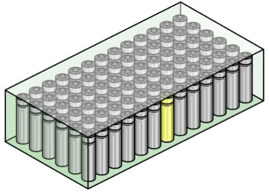
The battery cells are aligned into a modular section seen in Figure 2 below. The module dimensions are given as 1.5 x 0.8 x 0.0125 meters. The total number of battery cells in the module is given as 450, which with the discussed heat dissipation above produces a total of 2,250 Watts. It is presumed that the battery cells are sufficiently insulated from one another, directing the majority of heat dissipation towards the top of the module. As such, a finned heat sink is the ideal cooling method for this project.
Compared to other cooling systems, heat sinks have lower manufacturing costs, no moving parts or controlled fluids, and can be easily optimized for specific needs. As such, the preliminary cooling system investigated will be a finned heat sink with rectangular fins. Rectangular fins were chosen over other notable geometries (trapezoidal, triangular and cylindrical) because they are more common in standard manufacturing processes and have greater consistency in design manipulation and analysis. Therefore, this removes any variability associated with analytical validation. The materials considered for this heat sink were brass, copper alloys and aluminum alloys. After careful consideration, aluminum 6061 was chosen for a couple reasons. First, it has sufficient thermal properties compared to considered counterparts. Although it has lower thermal conductivity compared to copper alloys, aluminum 6061 is half the cost and has a lower mass. This is very important in racing vehicles.
Analytical Calculation
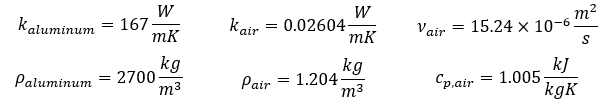
To begin the analytical analysis of the system, certain assumptions must be stated. First, battery cell insulation will be considered to be perfect, therfore, all dissipated heat will be applied to the heat sink. The bottom plate of the surface is then considered isothermal. It will also be assumed that there is negligible axial conduction of the heat sink and the heat sink fins are adiabatic. Finally, material and fluid properties are assumed to be constant. These properties are shown below.
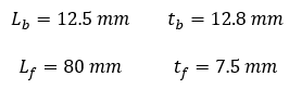
For analytical calculation, a heat sink is generated with sample dimensions shown below. These dimensions are used to compare analytical and simulated results to ensure heat dissipation metrics are being met. During the parametric study and corresponding optimization, fin dimensions will vary.
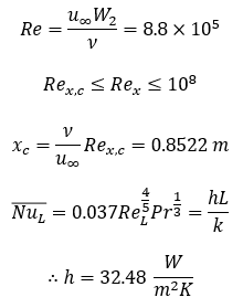
The first calculation is the coefficient of heat transfer for the air moving at 20 mph. The calculation will produce a coefficient for a flat plate boundary layer as shown in Figure 3 below.
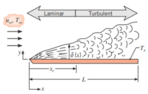
The Reynolds number for this flow is shown in Equation 1 below. Comparing this value to known flow correlations shown in Equation 2, the flow appears to have a mixed boundary layer at a location half the sink length. This can be seen in in Equation 3. To avoid transitioning boundary layers, the flow will be tripped prior to reaching the plate. Therefore, a turbulent boundary layer Nusselt number correlation is used which provides the estimated coefficient of heat transfer. This is shown in Equation 4 below.
To model the heat transfer of the heat sink, a resistance network is created as shown in Figure 4 below. As the heat rate from the battery cells is applied to the sink, the first resistance is the base plate Rt,base. As the heat flows outward, it is split between dissipation to outward air and the fins. This is modeled a resistances in parallel.
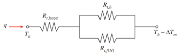
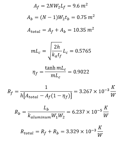
The equations to determine the resistance network can be found below. The efficiency of the fins is found by comparing the effectiveness of a fin with respect to the relationship between exposed base plate surface area to fin surface area. Equations 5, 6, and 7 calculate the area of the fin, area of the base and total area of the sink, respectively. The fin efficiency and fin resistance can be found by Equations 8 and 9. Equation 10 determines the resistance of the base plate. Finally, the total resistance of the sink is found by Equation 11.
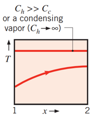
In many heat exchangers, as the cooling fluid moves through the fins it increases in temperature, lowering the heat transfer rate. Since the heat sink is long, it is assumed that constant heat transfer along the fin length is an inaccurate assumption. As a result, calculation must account for this decrease. To accomplish this, the NTU method is used. The NTU method determines the efficiency of a heat exchanger by defining the effectiveness as the ratio of actual heat transfer rate to the maximum possible heat transfer rate. Since the heat sink bottom surface temperature is considered spatially uniform and axial conduction is neglected, the heat sink behavior corresponds to that of a single stream heat exchanger. Specifically, the surface temperature does not vary in the x-direction, but the air temperature increases as it flows through the heat sink. This is illustrated in Figure 5 below.
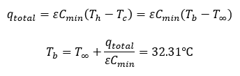
This calculation includes the heat capacity ratio of the hot and cold fluids. Since air is the only working fluid, the ratio is zero. This gives us the correlation for effectiveness, epsilon, shown in Equation 12 below. The minimum heat capacity rate, Cmin, can also be found by Equation 13. The heat capacity rate is related to the number of channels of sink, N, and the spacing, tb.
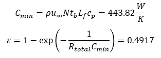
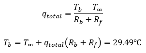
The heat dissipation of this exchanger including the heat capacity rate and assiciated effectiveness can be found in Equation 13 below. The temperatures Th and Tc refer to the hot and cold temperatures of the exchanger. For this case, the hot temperature is the temperature of the baseplate and the cold temperature is the ambient air temperature at the inlet of the sink. The heat dissipation rate, qtotal, can be replaced by the known heat generation rate of the battery cells to ensure module heat removal needs are met. The equation can then be rearranged for the base plate temperature, Tb, which is assumed to be the relative temperature of the battery cells. This specific sink geometry reaches a battery steady-state temperature of 32.31C, a value within the desired temperature range.
Thermal Simulation
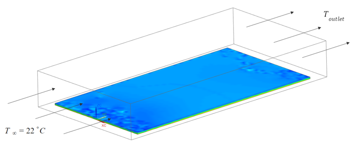
In order to validate analytical calculation, a simulation of the proposed heat sink was created. A sample flow chamber was created with the specified dimensions listed above. This can be seen in Figure 6 below. This simulation does not contain fins and as expected reaches steady-state at a temperature value well above the desired range. This temperature was determined to be 78.483C.
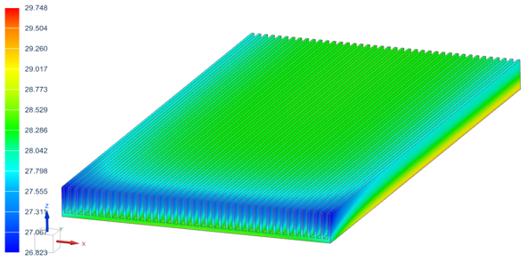
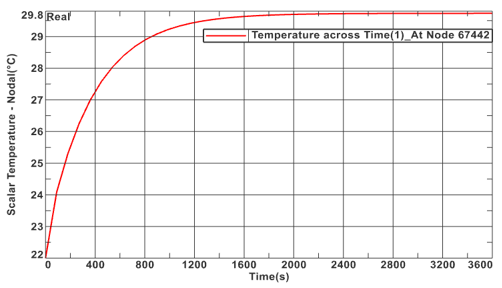
With the flow chamber completed, the simulation of the designed heat sink can be run. The steady-state simulation of the heat sink after the total 60 minute requirement can be found in Figure 7 below. During operation, as the ambient air increases in temperature the critical temperature region of the sink would occur in the back middle section. As a result, if this region remains within the temperature range all other sections would reside in the temperature range. Figure 8 shows the transcient temperature change of this region as it reaches steady-state. This final temperature is determined to be 29.784C.
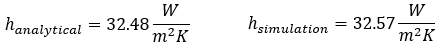
To verify the analytical and simulated values, the generated heat transfer coefficients are compared. The similation and analytical values are very similar, validating both the analytical and simulation solutions. Both values can be found below.
It can be noted, however, that the maximum temperature of the simulated results is lower than that of the analytical calculation. This difference is due to the assumption made by the simulation that the fluid temperature does not change along the x-direction. This issue was accounted for analytically by the aforementioned NTU method. In the simulation, the resistance network is modeled as a series system as shown in Figure 9 below.
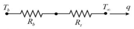
As such, the losses in fin efficiency are not accounted for resulting in a lower module temperature. The equation for heat dissipation is reduced to Equation 14 below. Similar to previous calculation, this is then rearranged for module temperature, tb, which produces a temperature of 29.49C. This reduced network returns a final temperature very similar to the simulation temperature of 29.78C as shown above. This simplified resistance model proves simulation validity, however, this temperature difference is significant in highlighting the importance of careful system assumptions.
Optimization and Parametric Study
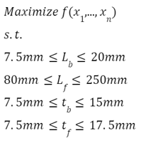
The purpose of optimization and parametric analysis is to determine the effect of variables, both geometric and environmental, on the system to optimize performance. In this project, certain parameters were assumed constant and therefore do not account for changes in operation conditions. First, the initial heat sink dimensions were created at random and are not necessarily ideal for the system at hand. To account for this, optimization of the heat sink geometry is completed. In order to remain within specified boundary conditions, upper and lower bounds are chosen for the fin dimensions. These bounds can be found in Figure 10 below and are base length, fin length, base thickness, and fin thickness.
To determine the impact of specific parameters relative to eachother, a parametric study is first completed. This not only provides insight into parameter impact but will later verify optimization results given the geometric parameters returned coinside with parametric trends. In order to generate values, a latin hypercube design space (LHS) is created and scaled for the design variables. LHS design was chosen over Monte Carlo design (MCS) due to superior randomness through statistical manipulation. The parametric study and optimization will be completed by a MATLAB script. After the LHS array is created, the values are used to complete the analytical calculation described above. For each specific property, all others are kept constant. The geometric changes and their respective effect on module temperature can be found in Figure 11 below.
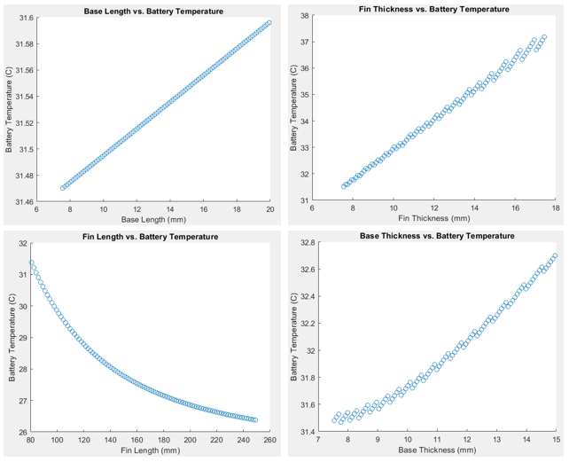
A few trends can be noticed from the study. First, the module temperature increases proportionally with base length and decreases asymptotically with fin length. This is caused by the relationship between conduction and convection. The Biot number (Bi) gives a simple index of the ratio of the thermal resistances inside of a body and at the surface of a body. If the Biot number is small (Bi << 1), the conduction within a body is considered orders of magnitude faster than convection, hence, the gradient of temperature is assumed uniform on the interior of the body. In this case, the Biot number is small as Bi ~ 0.19Lc. Therefore, conduction along the fin length dominates and the ratio between base length convection and fin length convection is small. This can also been seen in the effect of increasing thicknesses for the base plate and fins. The increased thicknesses does not improve transfer from the battery module to the cooling fluid but rather increases the stored energy of the heat sink. This does not have a large effect with small dimensions but as the dimensions get larger the negative effects grow. It should be noted that given the constraints of the heat sink width and length could create potential tolerancing issues with calculation. To prevent this, the increased dimensions may change the number of fins along the sink width. This explains why as the base thickness increases the battery temperature grows exponentially whereas the fin thickness only grows linearly. This also explains the discontinuities of the graphs. Regardless of this tolerancing prevention, the small continuous segments all have positive slopes of equal value. This proves that the increasing thicknesses are detrimental to sink performance, regardless of the overall trend slope.
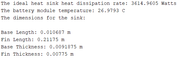
The completion of the parametric study leads to the optimization of the heat sink. Figure 11 below shows the output of the previously described MATLAB script. The script generates the LHS design space and then completes the analytical calculation described above to determine the heat dissipation rate of the sink and the final temperature of the battery module. The maximum heat dissipation rate and minimum battery module temperature are then provided with the associated heat sink geometric parameters. From the output below, it can be shown that the best heat sink dimensions result in a heat dissipation rate greater than required and a module temperature within the specified range. The dimensions of the heat sink also coinside with the geometric trends determined during the parametric study discussed above. This further affirms the validity of the result.
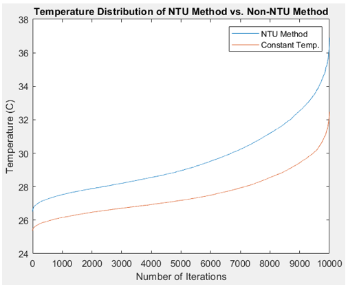
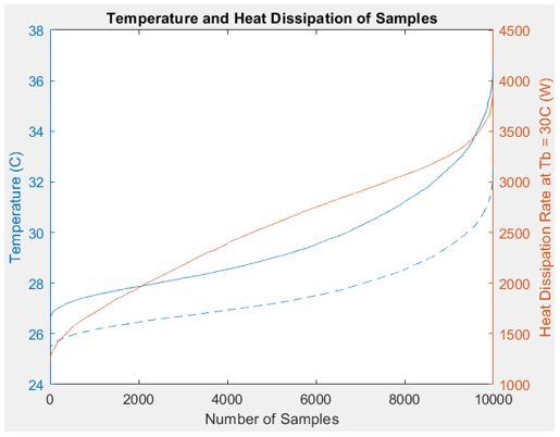
The effectiveness of the heat sink by the NTU method can also be shown in Figure 12 below. This plot shows the module temperature accounting for heat sink effectiveness (NTU) and maximum possible heat transfer rate. As previously discussed, the NTU method is a more accurate representation of the module temperature and prevents potential design oversight. It can be seen from this plot that this difference is around 2C and grows to 4C as the heat sink efficiency goes down. Assuming a more efficient heat sink is chosen, the non-NTU method still produces inaccurate temperatures 2C lower than ideal. A error that is likely to grow with changing environmental and operation conditions. Another plot provided is the module temperature and heat dissipation seen by Figure 13. This plot does not provide any specific insight, however, it does show that between ~2,000 and ~6,000 samples the heat dissipation grows and levels out as the module temperature levels and then grows. This may indicate areas where ideal parameters can be found.
Although the previous result is the ideal heat sink, it does not take into account the associated cost of material. In order to determine a heat sink that maximizes the performance relative to material cost, a cost effective ratio is generated. This ratio compares the heat dissipation rate of a sink to its cost of material by volume. This parameter allows the code to produce a heat sink with dimensions that produce results that adhere to minimum design specifications. Although results will barely meet desired specs, this allows for tailoring of the heat sink dimensions based on geometric trends seen in the parametric study. This can be seen in Figure 14 below.
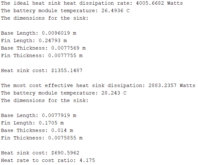
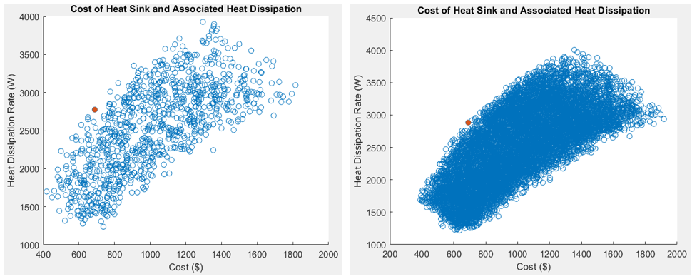
The ideal heat sink shown in this output produces close to double the required minimum heat dissipation and costs ~35% more than the allowed budget. The most cost effective heat sink dissipates ~28% more heat than what is required and costs ~30% less than the allowed budget. The benefit of this analysis is that is produces a cost effective heat sink that can be modified for desired specifications. For example, if the desired possible heat sink dissipation is 3,000 Watts, the parameters can be adjusted according to the geometric trends with minimal addition to cost. This is because the parameters are not changing together but individually in a controlled way. This result can also be seen in Figure 15 below. This plot is split into two sections, one with n = 1,000 samples and one with n = 10,000 samples. There is no specific reasoning other than to show the shape of the potential function area. In these plots, the heat dissipation and associated cost are compared. It can be assumed that the most ideal heat sinks would be closer to and higher up on the y-axis. This is indeed the case and the ideal value discussed in Figure 14 above is shown below in red.
Potential Sources of Error
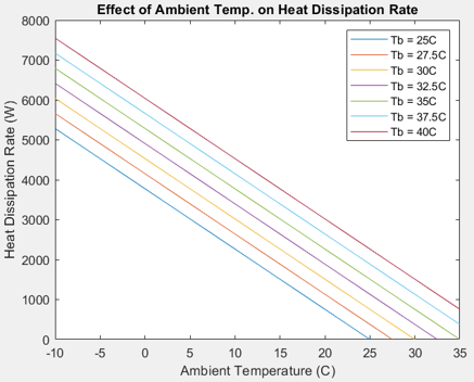
Althoug meeting project requirements, certain factors were simplified. For example, the constant battery C-rate and heat rate applied to the heat sink are averages during operation and do not reflect critical cases. Furthermore, no consideration of motor cooling was done nor the effect of non-geometric factors. These factors may lead to critical stress situations where battery temperatures rise above the desired range, reducing efficiency and harming battery life. Therefore, investigation into environmental effects are needed. The initial set temperature of the ambient air was 25C, a value that is highly variable during competition. Analyzing the changes in air temperature with constant air flow rate and set module temperature, we can see that the heat dissipation is linear in Figure 16 below. This outcome is expected and demonstrates the decreasing efficiency of the heat sink as the ambient conditions get worse. This also indicates that certain conditions do not produce required heat dissipation for the module of 2,250 Watts, a problem that can be solved if the flow rate is variable.
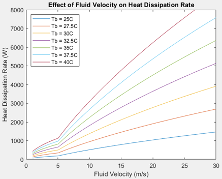
Considering the changes in air flow velocity, Figure 17 illustrates the effect of flow rate on the heat dissipation of the sink at various module temperature conditions shown in Figure 16 above. From this graph, it can be seen that prior to 5m/s the fluid is laminar and has insufficient heat dissipation regardless of ambient temperature. After the transition regions occurs, the flow breaks to turbulent and greater dissipation slopes can be seen. Previously set flow speed of 8.9m/s was based on average vehicle speeds during competition, however, this is not a dependable value as can be seen from the plot. If desired module temperature is set to 30C, flow must achieve ~15m/s which is double the average value. To combat this, flow should be tripped prior to reaching the plate to guarantee greater coefficient of heat transfer and dissipation.
Conclusion
In this study, a heat sink was selected as the cooling method for the module battery pack. Geometric parameters were compared and optimized for the given situation including a cost effective version that stayed well below the allocated budget. Although the selected version is ideal for the given situation, it is clear that a more robust thermal management system is needed to meet operation needs. This decisions coincides with the fact that no analysis was completed on the motor cooling nor other aspects of the vehicle. This system may be ideal for the battery pack alone, however, it may change in order to meet the cooling needs of these other components. A more robust cooling system is being designed as part of the Rensselaer Motorsport team. Please view that project to learn more about the developments in the cooling system.
References
[1] Bergman, T.L., Lavine, S.A., Incropera, F.P. and Dewitt, D.P. (2011) Fundamentals of Heat and Mass Transfer. 7th Edition, John Wiley & Sons, Hoboken.
[2] Nigel. "Heat Generation in a Cell." Battery Design, 24 Jan. 2022, https://www.batterydesign.net/heat-generation-in-a-cell/.
[3] Tie, S.F.; Tan, C.W. A review of energy sources and energy management system in electric vehicles. Renew. Sustain. Energy Rev. 2013
[4] Arora, S.; Shen, W.; Kapoor, A. Review of mechanical design and strategic placement technique of a robust battery pack for electric vehicles. Renew. Sustain. Energy Rev. 2016